from datetime import timedelta
from scipy import stats
from sklearn.preprocessing import RobustScaler
from sklearn.cluster import KMeans
from sklearn.metrics import silhouette_score

import chardet as cd
import pandas as pd
import seaborn as sb
import matplotlib.pyplot as plot
import plotly.express as px
import plotly.io as pio; pio.renderers.default = 'notebook'
import numpy as np数据来源:2010-2011 年间英国某在线零售商的所有真实交易
其中包含一家英国在线零售商在 2010 年 12 月 1 日至 2011 年 12 月 9 日期间发生的所有交易。该公司主要销售全场合礼品,且许多客户都是批发商。
数据准备
引入需要的库。
推断数据编码。
# detect the encoding
with open('./dataset/data.csv', 'rb') as raw_data:
    encoding_detected = cd.detect(raw_data.read(20000))
print(encoding_detected)
{'encoding': 'Windows-1252', 'confidence': 1.0, 'language': 'en'}读取数据。最好此时就把可能是 ID 的列指定为 str 类型,不然后续处理会比较麻烦,提前处理是一个性价比比较高的实践。
# read the dataset
data_origin = pd.read_csv('./dataset/data.csv', encoding=encoding_detected['encoding'], dtype={'CustomerID': str,'InvoiceNo': str})
display(data_origin)| InvoiceNo | StockCode | Description | Quantity | InvoiceDate | UnitPrice | CustomerID | Country | |
|---|---|---|---|---|---|---|---|---|
| 0 | 536365 | 85123A | WHITE HANGING HEART T-LIGHT HOLDER | 6 | 12/1/2010 8:26 | 2.55 | 17850 | United Kingdom |
| 1 | 536365 | 71053 | WHITE METAL LANTERN | 6 | 12/1/2010 8:26 | 3.39 | 17850 | United Kingdom |
| 2 | 536365 | 84406B | CREAM CUPID HEARTS COAT HANGER | 8 | 12/1/2010 8:26 | 2.75 | 17850 | United Kingdom |
| 3 | 536365 | 84029G | KNITTED UNION FLAG HOT WATER BOTTLE | 6 | 12/1/2010 8:26 | 3.39 | 17850 | United Kingdom |
| 4 | 536365 | 84029E | RED WOOLLY HOTTIE WHITE HEART. | 6 | 12/1/2010 8:26 | 3.39 | 17850 | United Kingdom |
| ... | ... | ... | ... | ... | ... | ... | ... | ... |
| 541904 | 581587 | 22613 | PACK OF 20 SPACEBOY NAPKINS | 12 | 12/9/2011 12:50 | 0.85 | 12680 | France |
| 541905 | 581587 | 22899 | CHILDREN'S APRON DOLLY GIRL | 6 | 12/9/2011 12:50 | 2.10 | 12680 | France |
| 541906 | 581587 | 23254 | CHILDRENS CUTLERY DOLLY GIRL | 4 | 12/9/2011 12:50 | 4.15 | 12680 | France |
| 541907 | 581587 | 23255 | CHILDRENS CUTLERY CIRCUS PARADE | 4 | 12/9/2011 12:50 | 4.15 | 12680 | France |
| 541908 | 581587 | 22138 | BAKING SET 9 PIECE RETROSPOT | 3 | 12/9/2011 12:50 | 4.95 | 12680 | France |
541909 rows × 8 columns
数据集包含约 54 万行记录,8 列或者说 8 个维度。
下一步需要初步处理重复值、缺失值和数据类型的问题。为后续的数据探索和特征工程等做准备。
处理重复值
当前业务场景下,不太可能会出现内容完全一致的记录,所以重复的记录可以认为是非法记录,需要删除。
# handle the duplicated values
count_duplicated = data_origin.duplicated().sum()
data_origin.drop_duplicates(inplace=True)
print(f'{count_duplicated} duplicated entries been dropped.')
5268 duplicated entries been dropped.处理缺失值
检查各个维度的缺失率。
# handle the null value
count_null = data_origin.isna().sum()
pd.DataFrame({
    'null(n)': count_null,
    'null(%)': round(((count_null / data_origin.count()) * 100), 1)
}).T| InvoiceNo | StockCode | Description | Quantity | InvoiceDate | UnitPrice | CustomerID | Country | |
|---|---|---|---|---|---|---|---|---|
| null(n) | 0.0 | 0.0 | 1454.0 | 0.0 | 0.0 | 0.0 | 135037.0 | 0.0 |
| null(%) | 0.0 | 0.0 | 0.3 | 0.0 | 0.0 | 0.0 | 33.6 | 0.0 |
从语义上讲,CustomerID 无法以任何方式进行推断填充。所以把此列为空的行直接删除。
# drop the rows with null CustomerID
count_null_customer_id = count_null['CustomerID']
data_origin.dropna(subset=['CustomerID'], inplace=True)
print(f'{count_null_customer_id} entries with null CustomerID been dropped.')

count_null = data_origin.isna().sum()
pd.DataFrame({
    'null(n)': count_null,
    'null(%)': round(((count_null / data_origin.count()) * 100), 1)
}).T
135037 entries with null CustomerID been dropped.| InvoiceNo | StockCode | Description | Quantity | InvoiceDate | UnitPrice | CustomerID | Country | |
|---|---|---|---|---|---|---|---|---|
| null(n) | 0.0 | 0.0 | 0.0 | 0.0 | 0.0 | 0.0 | 0.0 | 0.0 |
| null(%) | 0.0 | 0.0 | 0.0 | 0.0 | 0.0 | 0.0 | 0.0 | 0.0 |
现在所有维度都是非空的。
处理数据类型
检查各个维度的数据类型。
# check dtypes
data_origin.dtypes
InvoiceNo str
StockCode str
Description str
Quantity int64
InvoiceDate str
UnitPrice float64
CustomerID str
Country str
dtype: objectInvoiceDate 应该是日期。
data_origin['InvoiceDate'] = pd.to_datetime(data_origin['InvoiceDate'])
data_origin.dtypes
InvoiceNo str
StockCode str
Description str
Quantity int64
InvoiceDate datetime64[us]
UnitPrice float64
CustomerID str
Country str
dtype: object初步数据清洗结束。现在还剩约 40 万条记录。
display(data_origin)| InvoiceNo | StockCode | Description | Quantity | InvoiceDate | UnitPrice | CustomerID | Country | |
|---|---|---|---|---|---|---|---|---|
| 0 | 536365 | 85123A | WHITE HANGING HEART T-LIGHT HOLDER | 6 | 2010-12-01 08:26:00 | 2.55 | 17850 | United Kingdom |
| 1 | 536365 | 71053 | WHITE METAL LANTERN | 6 | 2010-12-01 08:26:00 | 3.39 | 17850 | United Kingdom |
| 2 | 536365 | 84406B | CREAM CUPID HEARTS COAT HANGER | 8 | 2010-12-01 08:26:00 | 2.75 | 17850 | United Kingdom |
| 3 | 536365 | 84029G | KNITTED UNION FLAG HOT WATER BOTTLE | 6 | 2010-12-01 08:26:00 | 3.39 | 17850 | United Kingdom |
| 4 | 536365 | 84029E | RED WOOLLY HOTTIE WHITE HEART. | 6 | 2010-12-01 08:26:00 | 3.39 | 17850 | United Kingdom |
| ... | ... | ... | ... | ... | ... | ... | ... | ... |
| 541904 | 581587 | 22613 | PACK OF 20 SPACEBOY NAPKINS | 12 | 2011-12-09 12:50:00 | 0.85 | 12680 | France |
| 541905 | 581587 | 22899 | CHILDREN'S APRON DOLLY GIRL | 6 | 2011-12-09 12:50:00 | 2.10 | 12680 | France |
| 541906 | 581587 | 23254 | CHILDRENS CUTLERY DOLLY GIRL | 4 | 2011-12-09 12:50:00 | 4.15 | 12680 | France |
| 541907 | 581587 | 23255 | CHILDRENS CUTLERY CIRCUS PARADE | 4 | 2011-12-09 12:50:00 | 4.15 | 12680 | France |
| 541908 | 581587 | 22138 | BAKING SET 9 PIECE RETROSPOT | 3 | 2011-12-09 12:50:00 | 4.95 | 12680 | France |
401604 rows × 8 columns
探索数据内容
这一步的目的是理解数据集的各个维度的语义和内容,根据语义进一步剔除非法记录,并初步洞察数据集。
业务语义探索
数据集有 8 个维度。根据列名初步推测业务语义:
InvoiceNo:发票号。分配给每笔交易的唯一编码。StockCode:产品(商品)代码。分配给每种产品的唯一编码。Description:产品(条目)名称。Quantity:每次交易每种产品(商品)的数量。InvoiceDate:每笔交易生成的日期和时间。UnitPrice:单价。每单位产品价格(以英镑为单位)。CustomerID:客户编号。分配给每个客户的 5 位唯一整数编码。Country:国家名称。每个客户居住的国家/地区的名称。
InvoiceNo
现阶段可以假设 InvoiceNo 是一个 6 位流水号,每个流水号代表一笔订单。
# check if InvoiceNO a fixed 6 width number
value_counts_invoice_no_len = data_origin['InvoiceNo'].str.len().value_counts()

pd.DataFrame({
    'n': value_counts_invoice_no_len,
    '%': round((value_counts_invoice_no_len / len(data_origin) * 100), 1)
}).T| InvoiceNo | 6 | 7 |
|---|---|---|
| n | 392732.0 | 8872.0 |
| % | 97.8 | 2.2 |
假设失败,InvoiceNo 是 6 位或者 7 位。
value_counts_invoice_no_isnumeric = data_origin['InvoiceNo'].str.isnumeric().value_counts()

pd.DataFrame({
    'n': value_counts_invoice_no_isnumeric,
    '%': round((value_counts_invoice_no_isnumeric / len(data_origin) * 100), 1)
}).T| InvoiceNo | True | False |
|---|---|---|
| n | 392732.0 | 8872.0 |
| % | 97.8 | 2.2 |
且 InvoiceNo 也并不全由数字组成。
mask_7_len_invoice_no = data_origin['InvoiceNo'].str.len() == 7
mask_numeric_invoice_no = data_origin['InvoiceNo'].str.isnumeric()
(mask_7_len_invoice_no != ~mask_numeric_invoice_no).sum()np.int64(0)经验证。所有 7 位 InvoiceNo 的记录与不是纯数字的 InvoiceNo 的记录一致。
浏览这些 7 位 InvoiceNo 记录。
data_origin[mask_7_len_invoice_no]| InvoiceNo | StockCode | Description | Quantity | InvoiceDate | UnitPrice | CustomerID | Country | |
|---|---|---|---|---|---|---|---|---|
| 141 | C536379 | D | Discount | -1 | 2010-12-01 09:41:00 | 27.50 | 14527 | United Kingdom |
| 154 | C536383 | 35004C | SET OF 3 COLOURED FLYING DUCKS | -1 | 2010-12-01 09:49:00 | 4.65 | 15311 | United Kingdom |
| 235 | C536391 | 22556 | PLASTERS IN TIN CIRCUS PARADE | -12 | 2010-12-01 10:24:00 | 1.65 | 17548 | United Kingdom |
| 236 | C536391 | 21984 | PACK OF 12 PINK PAISLEY TISSUES | -24 | 2010-12-01 10:24:00 | 0.29 | 17548 | United Kingdom |
| 237 | C536391 | 21983 | PACK OF 12 BLUE PAISLEY TISSUES | -24 | 2010-12-01 10:24:00 | 0.29 | 17548 | United Kingdom |
| ... | ... | ... | ... | ... | ... | ... | ... | ... |
| 540449 | C581490 | 23144 | ZINC T-LIGHT HOLDER STARS SMALL | -11 | 2011-12-09 09:57:00 | 0.83 | 14397 | United Kingdom |
| 541541 | C581499 | M | Manual | -1 | 2011-12-09 10:28:00 | 224.69 | 15498 | United Kingdom |
| 541715 | C581568 | 21258 | VICTORIAN SEWING BOX LARGE | -5 | 2011-12-09 11:57:00 | 10.95 | 15311 | United Kingdom |
| 541716 | C581569 | 84978 | HANGING HEART JAR T-LIGHT HOLDER | -1 | 2011-12-09 11:58:00 | 1.25 | 17315 | United Kingdom |
| 541717 | C581569 | 20979 | 36 PENCILS TUBE RED RETROSPOT | -5 | 2011-12-09 11:58:00 | 1.25 | 17315 | United Kingdom |
8872 rows × 8 columns
data_origin[mask_7_len_invoice_no]['InvoiceNo'].str[0].value_counts()InvoiceNo
C 8872
Name: count, dtype: int64所有 7 位 InvoiceNo 的前缀都是 “C”。
(data_origin[mask_7_len_invoice_no]['Quantity'] < 0).sum()np.int64(8872)所有 7 位 InvoiceNo 的 Quantity 都小于 0。
可以推测,所有以 “C” 开头的 7 位 InvoiceNo 代表的记录,都表示这个订单已经被取消,所以用负值 Quantity 来冲抵。
如果是这样,那么这部分被取消的记录一定有对应的正向销售记录。
# check if ‘C’ means ‘Cancel’
data_test_cancel = data_origin[['StockCode', 'Quantity', 'InvoiceDate', 'CustomerID']]
data_test_cancel.sort_values(by=['CustomerID', 'StockCode', 'InvoiceDate'])
data_test_cancel['StockCumSum'] = data_test_cancel.groupby(['CustomerID', 'StockCode'])['Quantity'].cumsum()

def verify_row(row):
    if row['Quantity'] >= 0:
        return 'Normal Sale'
    elif row['StockCumSum'] >= 0:
        return 'Valid Return'
    else:
        return 'Orphan/Excess Return'

data_test_cancel['ValidationStatus'] = data_test_cancel.apply(verify_row, axis='columns')
count_status = data_test_cancel['ValidationStatus'].value_counts()
pd.DataFrame({
    'n': count_status,
    '%': round(((count_status / len(data_test_cancel)) * 100), 1)
}).T| ValidationStatus | Normal Sale | Valid Return | Orphan/Excess Return |
|---|---|---|---|
| n | 392732.0 | 7462.0 | 1410.0 |
| % | 97.8 | 1.9 | 0.4 |
8872 条记录中,有 7462 条正常取消的记录,还有 1410 条没有正向销售记录,可能是由于对应的正向销售记录在数据集更往前的时间。
考虑到没有正向销售记录的仅占 0.4%,不再继续深究,直接把这部分记录删除。
# drop orphan orders
mask_orphan_orders = data_test_cancel['ValidationStatus'] == 'Orphan/Excess Return'
orphan_orders = data_origin[mask_orphan_orders]
data_origin.drop(index=orphan_orders.index, inplace=True)
print(f'{len(orphan_orders)} orphan entries been dropped.')
1410 orphan entries been dropped.综上,InvoiceNo 整体上是一个 6 位数字流水号,但是当它以 “C” 开头,变成 7 位时,代表这条交易记录已经被取消。
StockCode
现阶段可以假设 StockCode 是一个 5 位产品(商品)代码,但是以字母结尾,变成 6 位时,代表了某种语义。
value_counts_stock_code_len = data_origin['StockCode'].str.len().value_counts()

pd.DataFrame({
    'n': value_counts_stock_code_len,
    '%': round((value_counts_stock_code_len / len(data_origin) * 100), 3)
}).T| StockCode | 5 | 6 | 4 | 1 | 7 | 2 | 3 | 12 |
|---|---|---|---|---|---|---|---|---|
| n | 365177.00 | 33097.00 | 1143.000 | 320.00 | 295.000 | 134.000 | 16.000 | 12.000 |
| % | 91.25 | 8.27 | 0.286 | 0.08 | 0.074 | 0.033 | 0.004 | 0.003 |
假设失败,StockCode 有 1~7 位和 12 位。但是绝大部分是 5 位。
data_origin[data_origin['StockCode'].str.len() == 5]['StockCode'].str.isnumeric().sum()np.int64(365177)所有 5 位 StockCode 都是纯数字编码。
data_origin[data_origin['StockCode'].str.startswith('15044')][['StockCode', 'Description']].drop_duplicates()| StockCode | Description | |
|---|---|---|
| 1097 | 15044B | BLUE PAPER PARASOL |
| 12970 | 15044C | PURPLE PAPER PARASOL |
| 40154 | 15044A | PINK PAPER PARASOL |
| 59815 | 15044D | RED PAPER PARASOL |
任意抽了一个 6 位编码,看起来不同字母后缀的 StockCode 代表了同一产品的不同款式。
data_origin[data_origin['StockCode'].str.len().between(1, 4)][['StockCode', 'Description']].value_counts()StockCode Description
POST POSTAGE 1139
M Manual 320
C2 CARRIAGE 134
DOT DOTCOM POSTAGE 16
PADS PADS TO MATCH ALL CUSHIONS 4
Name: count, dtype: int641 ~ 4 位 StockCode 分别表示:
POST,表示邮费PADS,表示包装用的垫子费用DOT,表示在线邮费C2,表示运费M,表示手动录入的特殊费用
客户在前端网站下单购买时,运费用 DOT,经销商大宗运输时,运费用 C2,小批量补发商品时,用 POST
data_origin[data_origin['StockCode'].str.len() == 12]['StockCode'].value_counts()StockCode
BANK CHARGES 12
Name: count, dtype: int64所有 12 位 StockCode 都是 BANK CHARGES,表示银行收取的交易费用。
综上,StockCode 有多种形式:
- 5 位数字(+ 1 位字母)编码,表示一款产品
D、M、C2、DOT、PADS、POST、BANK CHARGES分别代表附带的特殊费用或折扣
其他维度
按照语义来讲,预期 Quantity 和 UnitPrice 应该呈现右偏分布。
fig, axis = plot.subplots(nrows=1, ncols=2, figsize=(12, 5))

mask_product_sale = (data_origin['Quantity'] > 0) & data_origin['StockCode'].str.len().between(5,6)
data_product_sale = data_origin[mask_product_sale]

q1_of_quantity = data_product_sale['Quantity'].quantile(0.25)
q3_of_quantity = data_product_sale['Quantity'].quantile(0.75)
iqr_of_quantity = q3_of_quantity - q1_of_quantity
mask_no_outlier_quantity = data_product_sale['Quantity'] <= q3_of_quantity + 1.5 * iqr_of_quantity

q1_of_unit_price = data_product_sale['UnitPrice'].quantile(0.25)
q3_of_unit_price = data_product_sale['UnitPrice'].quantile(0.75)
iqr_of_unit_price = q3_of_unit_price - q1_of_unit_price
mask_no_outlier_unit_price = data_product_sale['UnitPrice'] <= q3_of_unit_price + 1.5 * iqr_of_unit_price

hist_quantity = sb.histplot(data_product_sale[mask_no_outlier_quantity]['Quantity'], ax=axis[0], bins='fd', kde=True, discrete=True)
hist_unit_price = sb.histplot(data_product_sale[mask_no_outlier_unit_price]['UnitPrice'], ax=axis[1], bins='fd', kde=True)

hist_quantity.set_title('Distribution of Quantity')
hist_unit_price.set_title('Distribution of UnitPrice')

plot.tight_layout()
plot.show()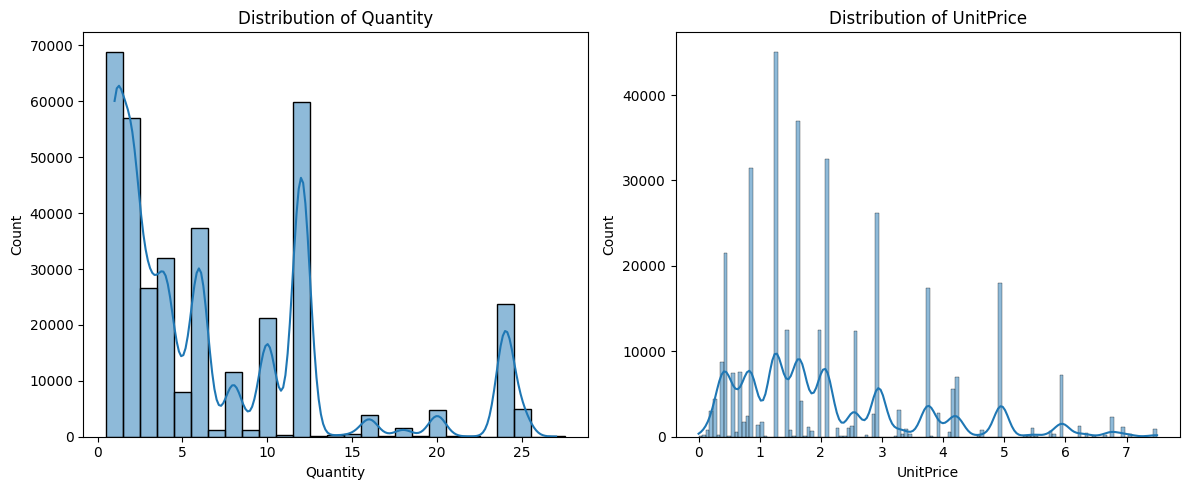
从图上看,大体符合预期。
data_origin['CustomerID'].str.len().value_counts()CustomerID
5 400194
Name: count, dtype: int64data_origin['CustomerID'].str.isnumeric().value_counts()CustomerID
True 400194
Name: count, dtype: int64CustomerID 是一个 5 位数字。
data_origin['Country'].value_counts()Country
United Kingdom 355446
Germany 9422
France 8462
EIRE 7453
Spain 2524
Netherlands 2369
Belgium 2068
Switzerland 1877
Portugal 1468
Australia 1255
Norway 1083
Italy 797
Channel Islands 756
Finland 695
Cyprus 610
Sweden 460
Austria 400
Denmark 389
Japan 355
Poland 341
USA 291
Israel 245
Unspecified 241
Singapore 227
Iceland 182
Canada 151
Greece 146
Malta 126
United Arab Emirates 68
European Community 61
RSA 58
Lebanon 45
Lithuania 35
Brazil 32
Czech Republic 29
Bahrain 17
Saudi Arabia 10
Name: count, dtype: int64Country 看起来没有 Typo 问题。
value_counts_country = data_origin['Country'].value_counts().reset_index()
value_counts_country.columns = ['Country', 'Count']

fig = px.choropleth(value_counts_country,
                    locations='Country',
                    locationmode='country names',
                    color='Count',
                    hover_name='Country',
                    title='Distribution of Country')

fig.show()
C:\Users\z1197\AppData\Local\Temp\ipykernel_5168\4015351048.py:4: DeprecationWarning:
The library used by the *country names* `locationmode` option is changing in an upcoming version. Country names in existing plots may not work in the new version. To ensure consistent behavior, consider setting `locationmode` to *ISO-3*.
可以发现,英国的订单量远高于其他地区。考虑到数据集来自于英国商店,有其合理性。
分离退货订单和销售订单
现在的订单汇中,混杂了取消订单和销售订单。此处有两条处理思路:
- 考虑把退货订单匹配回原始销售订单,增加一个维度用于表示已经取消的商品数量,用于后续计算订单的真实价值
- 直接分离退货订单和销售订单,分开分析
此处我倾向于选择后者,因为退货订单可能无法精确匹配到原始订单,即使匹配,也可能存在部分退货、多次退货等复杂情况,分离分析避免了匹配错误带来的偏差。再者,购买行为代表客户的购买意愿和消费能力,退货行为代表客户满意度、产品质量问题、物流问题等,两者分开分析:可以更清晰地看到客户的真实行为模式。
mask_canceled = data_origin['InvoiceNo'].str.startswith('C')
data_canceled = data_origin[mask_canceled]
data = data_origin[~mask_canceled]
data_product_sale = data[data['InvoiceNo'].str.len().between(5, 6)]
特征工程
这一步的目的是把原始数据转换成便于进行 RFM 分群的样子。
data_product_sale['TotalAmount'] = data_product_sale['Quantity'] * data_product_sale['UnitPrice']
base_date = data_product_sale['InvoiceDate'].max() + timedelta(days=1)
data_rfm = data_product_sale.groupby('CustomerID').agg({
    'InvoiceDate': lambda x: (base_date - x.max()).days,
    'InvoiceNo': 'nunique',
    'TotalAmount': 'sum'
}).reset_index()
data_rfm.columns = ['CustomerID', 'Recency', 'Frequency', 'Monetary']
探索性数据分析
我将从三个维度展开 EDA:
- 单变量分析:检查 R、F、M 各自的分布特征
- 双变量分析:探索 R-F、R-M、F-M 之间的相关性
- 多变量分析:识别异常客户群体
# single variable analysis
fig, axis = plot.subplots(2, 3, figsize=(15, 10))

# Recency
sb.histplot(data=data_rfm, x='Recency', discrete=True, kde=True, ax=axis[0, 0])
axis[0, 0].set_title('Recency Distribution (Days since last purchase)')
axis[0, 0].axvline(data_rfm['Recency'].median(), color='red', linestyle='--',
                   label=f'Median: {data_rfm["Recency"].median():.0f} days')
axis[0, 0].legend()
sb.boxplot(data=data_rfm, x='Recency', ax=axis[1, 0])
axis[1, 0].set_title('Recency Boxplot')

# Frequency
sb.histplot(data=data_rfm, x='Frequency', discrete=True, kde=True, ax=axis[0, 1])
axis[0, 1].set_title('Frequency Distribution (Number of orders)')
# Frequency usually has a long tail
data_rfm['Frequency_log'] = np.log1p(data_rfm['Frequency'])
sb.histplot(data=data_rfm, x='Frequency_log', bins='fd', kde=True, ax=axis[1, 1])
axis[1, 1].set_title('Frequency Distribution (Log-transformed)')

# Monetary
sb.histplot(data=data_rfm, x='Monetary', bins=30, kde=True, ax=axis[0, 2])
axis[0, 2].set_title('Monetary Distribution (Total spending)')
# Monetary usually has a long tail
data_rfm['Monetary_log'] = np.log1p(data_rfm['Monetary'])
sb.histplot(data=data_rfm, x='Monetary_log', bins=30, kde=True, ax=axis[1, 2])
axis[1, 2].set_title('Monetary Distribution (Log-transformed)')

plot.tight_layout()
plot.show()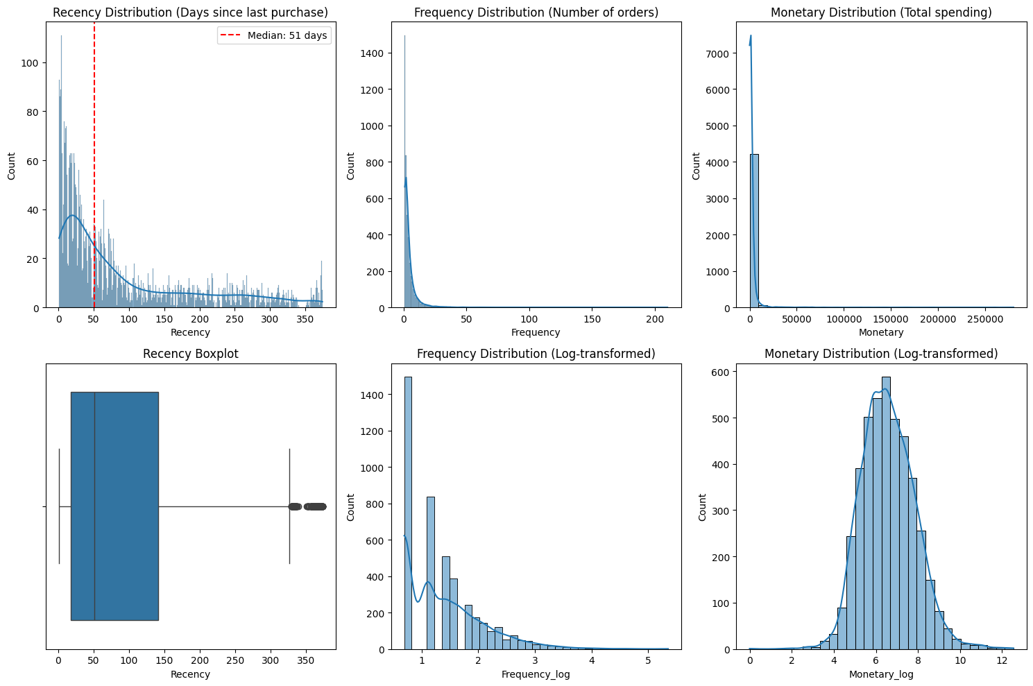
R 呈现明显的长尾分布。中位数为 51 天(红色虚线),意味着一半的客户在 51 天内有交易,但最右侧有接近 365 天未交易的客户。活跃客户占比较高,但存在明显的流失风险区间(长尾部分)。F 和 M 呈现极端严重的右偏态。绝大多数数据挤在靠近 0 的左侧,右侧有极长且稀疏的尾巴,此处存在“二八定律”,即极少数的“超级客户”贡献了绝大部分的订单量和销售额。如果不进行处理,这些离群值(Outliers)会严重干扰后续的聚类算法(如 K-Means)。
R 的箱线图中,中位线靠左,箱体较宽。右侧(350天附近)出现了一排黑点,这些是离群值,代表那些已经很久没有回访、极有可能已经彻底流失的客户。业务上可以将 51 天作为一个关键的流失预警节点。
# describe statistic
rfm_stats = data_rfm[['Recency', 'Frequency', 'Monetary']].describe()
rfm_stats.loc['skewness'] = data_rfm[['Recency', 'Frequency', 'Monetary']].apply(stats.skew)
rfm_stats.loc['kurtosis'] = data_rfm[['Recency', 'Frequency', 'Monetary']].apply(stats.kurtosis)
print("RFM Descriptive Statistics with Skewness and Kurtosis:")
rfm_stats
RFM Descriptive Statistics with Skewness and Kurtosis:| Recency | Frequency | Monetary | |
|---|---|---|---|
| count | 4339.000000 | 4339.000000 | 4339.000000 |
| mean | 92.518322 | 4.271952 | 2048.215924 |
| std | 100.009747 | 7.705493 | 8984.248352 |
| min | 1.000000 | 1.000000 | 0.000000 |
| 25% | 18.000000 | 1.000000 | 306.455000 |
| 50% | 51.000000 | 2.000000 | 668.560000 |
| 75% | 142.000000 | 5.000000 | 1660.315000 |
| max | 374.000000 | 210.000000 | 280206.020000 |
| skewness | 1.245926 | 12.095844 | 19.334716 |
| kurtosis | 0.429503 | 250.082433 | 478.234792 |
F 和 M 的偏度远大于 1,需要保留对数变换。
# correlation matrix
correlation_matrix = data_rfm[['Recency', 'Frequency', 'Monetary']].corr()
sb.heatmap(correlation_matrix, annot=True, cmap='coolwarm', center=0, square=True, linewidths=1)
plot.title('RFM Correlation Matrix')

plot.tight_layout()
plot.show()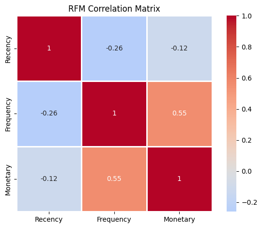
R 与 F 负相关(最近购买客户通常更活跃),F 与 M 正相关(购买次数多则总消费高),R 与 M 无明显相关性。
data_rfm_log = data_rfm[['Recency', 'Frequency_log', 'Monetary_log']].copy()
data_rfm_log.columns = ['Recency', 'Frequency (log)', 'Monetary (log)']
sb.pairplot(data_rfm_log, diag_kind='kde', plot_kws={'alpha': 0.5})
plot.suptitle('RFM Scatter Plot Matrix (with Log-transformed F & M)', y=1.02)

plot.tight_layout()
plot.show()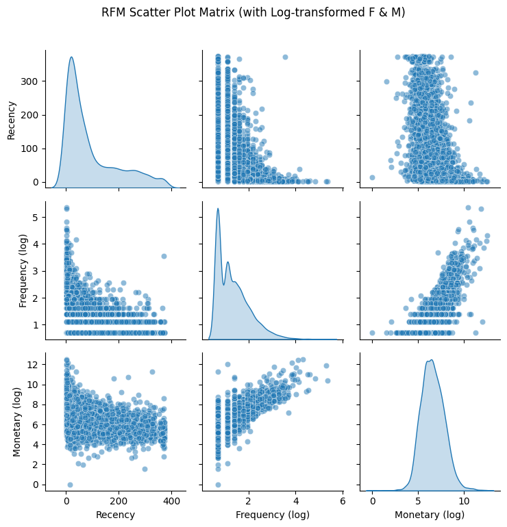
F 经过对数处理后,分布呈现多峰状态。左侧最高的峰表示大部分客户的消费频率较低(log 转换后数值较小),右侧的小峰则代表了高频活跃客户。
同时,F 和 M 这两个变量展现出极其显著的正相关关系。在图中可以看到散点呈线性向上排列。消费频率越高(F 越大)的客户,其贡献的总消费金额(M)通常也越高。这符合商业直觉,这类客户是企业的核心价值贡献者。R 和 F 的散点集中在 R 较低且 F 较低的区域,当 R 增加(距离上次消费时间变长)时,高频率消费的客户明显减少,这意味着高频客户如果长时间不来消费,流失风险极大。R 和 M 关系相对分散,但依然能看到 R 较小时,M 的高值点更多,这意味着最近有过消费的客户中,存在一部分高价值客户。随着 R 增加,高金额消费者的密度在下降。
# check if standardization needed
coefficient = data_rfm[['Recency', 'Frequency', 'Monetary']].std() / data_rfm[['Recency', 'Frequency', 'Monetary']].mean()
print(f'coefficient of variables:\n{coefficient}\n')
print(f'max cov / min cov = {coefficient.max() / coefficient.min():.3}')
coefficient of variables:
Recency 1.080972
Frequency 1.803740
Monetary 4.386378
dtype: float64
max cov / min cov = 4.06CV 值差异过大(> 2),在聚类分析(如K-Means)中,算法使用欧氏距离(\(\text{distance} = \sqrt{(x₁ - x₂)² + (y₁ - y₂)² + (z₁ - z₂)²}\))计算样本间相似度:如果特征尺度差异显著:
- Monetary 的 CV = 4.4 → 数据点在该维度上分布广泛(差异可达数千元)
- Recency 的 CV = 1.1 → 数据点在该维度上分布紧凑(差异可能只有几天)
假设两个客户比较:
- 客户A: Recency = 10 天, Monetary = 100 元
- 客户B: Recency = 20 天, Monetary = 10,000 元
欧氏距离计算:
- Recency 差异贡献: (10-20)² = 100
- Monetary 差异贡献: (100-10,000)² = 99,000,000
Monetary 的贡献是 Recency 的 990,000 倍!聚类结果将完全由 Monetary 主导,Recency 和 Frequency 的影响被忽略。
需要进行标准化处理,考虑到 Monetary 为极度右偏分布,选择对数化后用 RobustScalar 处理。
scalar = RobustScaler()
data_rfm_scaled = scalar.fit_transform(data_rfm[['Recency', 'Frequency_log', 'Monetary_log']])
data_rfm_scaled = pd.DataFrame(data_rfm_scaled, columns=['R_scaled', 'F_scaled', 'M_scaled'])
print("range after scaled:")
print(f"R_scaled    [{data_rfm_scaled['R_scaled'].min():.2f}, {data_rfm_scaled['R_scaled'].max():.2f}]")
print(f"F_scaled    [{data_rfm_scaled['F_scaled'].min():.2f}, {data_rfm_scaled['F_scaled'].max():.2f}]")
print(f"M_scaled    [{data_rfm_scaled['M_scaled'].min():.2f}, {data_rfm_scaled['M_scaled'].max():.2f}]")
print('------')
print(f'mean after scaled:\n{data_rfm_scaled.mean()}')
range after scaled:
R_scaled [-0.40, 2.60]
F_scaled [-0.37, 3.87]
M_scaled [-3.86, 3.58]
------
mean after scaled:
R_scaled 0.334825
F_scaled 0.224707
M_scaled 0.047671
dtype: float64sb.pairplot(data_rfm_scaled, diag_kind='kde', plot_kws={'alpha': 0.5})
plot.suptitle('Scaled-RFM Scatter Plot Matrix', y=1.02)
plot.tight_layout()
plot.show()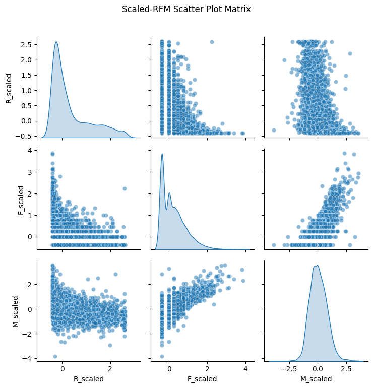
看着散点图没有发生明显变化,此次处理数据没有导致失真。
def evaluate_scaling_effectiveness(data_rfm_scaled):
    """evaluate scaling effectiveness"""
    evaluation = pd.DataFrame(index=['R_scaled', 'F_scaled', 'M_scaled'])

    for col in evaluation.index:
        data = data_rfm_scaled[col]

        # 基本统计量
        evaluation.loc[col, 'mean'] = data.mean()
        evaluation.loc[col, 'std'] = data.std()
        evaluation.loc[col, 'median'] = data.median()

        # 范围相关
        evaluation.loc[col, 'min'] = data.min()
        evaluation.loc[col, 'max'] = data.max()
        evaluation.loc[col, 'range'] = data.max() - data.min()
        evaluation.loc[col, 'IQR'] = np.percentile(data, 75) - np.percentile(data, 25)

        # 分布形状
        evaluation.loc[col, 'skewness'] = stats.skew(data)
        evaluation.loc[col, 'kurtosis'] = stats.kurtosis(data)

        # 理想值对比
        evaluation.loc[col, 'std_deviation'] = abs(data.std() - 1)  # 偏离1的程度
        evaluation.loc[col, 'mean_deviation'] = abs(data.mean())    # 偏离0的程度

        # 异常值比例(基于 1.5 * IQR 规则)
        Q1 = np.percentile(data, 25)
        Q3 = np.percentile(data, 75)
        IQR_val = Q3 - Q1
        bound_lower = Q1 - 1.5 * IQR_val
        bound_upper = Q3 + 1.5 * IQR_val
        mask_outlier = (data < bound_lower) | (data > bound_upper)
        evaluation.loc[col, 'outlier_pct'] = mask_outlier.mean() * 100

    return evaluation

evaluation_results = evaluate_scaling_effectiveness(data_rfm_scaled)
print("scaling result: ")
display(evaluation_results.round(4))
scaling result: | mean | std | median | min | max | range | IQR | skewness | kurtosis | std_deviation | mean_deviation | outlier_pct | |
|---|---|---|---|---|---|---|---|---|---|---|---|---|
| R_scaled | 0.3348 | 0.8065 | 0.0 | -0.4032 | 2.6048 | 3.0081 | 1.0 | 1.2459 | 0.4295 | 0.1935 | 0.3348 | 3.5723 |
| F_scaled | 0.2247 | 0.6218 | 0.0 | -0.3691 | 3.8715 | 4.2405 | 1.0 | 1.2085 | 1.6821 | 0.3782 | 0.2247 | 0.9680 |
| M_scaled | 0.0477 | 0.7482 | 0.0 | -3.8568 | 3.5783 | 7.4351 | 1.0 | 0.3636 | 0.8441 | 0.2518 | 0.0477 | 1.2215 |
| 指标 | R_scaled | F_scaled | M_scaled | 评估标准 | 结论 |
|---|---|---|---|---|---|
| 标准差 | 0.8065 | 0.6218 | 0.7482 | 差异<2倍 | 优秀 (最大/最小=1.30) |
| 偏度 | 1.246 | 1.209 | 0.364 | <1.5 | 可接受 |
| 均值偏差 | 0.335 | 0.225 | 0.048 | <0.5 | 良好 |
| 异常值比例 | 3.57% | 0.97% | 1.22% | <5% | 正常 |
| IQR | 1.0 | 1.0 | 1.0 | =1.0 | 符合预期 |
聚类敏感性测试
X_scaled = data_rfm_scaled[['R_scaled', 'F_scaled', 'M_scaled']].values

# test K=4 cluster
kmeans_test = KMeans(n_clusters=8, random_state=0, n_init=10)
labels = kmeans_test.fit_predict(X_scaled)

centers = kmeans_test.cluster_centers_
feature_importance = np.std(centers, axis=0)

print('cluster center features std:')
feature_names = ['Recency', 'Frequency', 'Monetary']
for i, (name, imp) in enumerate(zip(feature_names, feature_importance)):
    print(f"{name}: {imp:.4f}")

print('------')
importance_ratio = feature_importance.max() / feature_importance.min()
print(f"min/max feature importance ratio: {importance_ratio:.2f}")

# evaluate standard
if importance_ratio > 3:
    print("warning:some feature may over dominated")
elif importance_ratio > 2:
    print("warning:features contribution not balanced")
else:
    print("excellent:all features have a reasonable contribution")

print('------')
sil_score = silhouette_score(X_scaled, labels)
print(f"silhouette score: {sil_score:.4f}")

# evaluate standard
if sil_score > 0.5:
    print("good cluster structure")
elif sil_score > 0.25:
    print("normal cluster structure, result will need to be carefully explained")
else:
    print("bad cluster structure")
cluster center features std:
Recency: 0.8078
Frequency: 0.7305
Monetary: 0.8285
------
min/max feature importance ratio: 1.13
excellent:all features have a reasonable contribution
------
silhouette score: 0.2969
normal cluster structure, result will need to be carefully explained建模分析
现在正式开始建模分析。